# /!\/!\/!\ à exécuter si nécessaire
# install.packages("tidyverse", type = "win.binary")

# 0 - Nettoyer son env de travail
rm(list=ls())

# Charger librairies
library(dplyr)
library(sf)
library(leaflet)
library(ggplot2)
library(ggspatial)
library(osmdata)
library(tidyr)
library(readxl)

# 0 -Fixer le repertoire de travail
setwd("~/git/MASTER_1_R/data")

# 1 - Ouvrir les donnees
communes <- st_read("communes_vulnerables_polygn_5490.shp", quiet=T)
irisDfPop <- read_excel("base-ic-evol-struct-pop-2017.xlsx", sheet = "IRIS", skip = 5)
irisDfAct <-  read_excel("base-ic-activite-residents-2017.xlsx", sheet = "IRIS", skip = 5)

# 2 - Filtrer les donnees INSEE
irisDfPop <- irisDfPop %>%
  filter(LIBCOM %in% communes$NOM)
irisDfAct <- irisDfAct %>%
  filter(LIBCOM %in% communes$NOM)
Visualisation interactive avec Leaflet
# 3 - Afficher les communes sur une carte
leaflet() %>%
  addProviderTiles("Esri.WorldImagery") %>%
  addPolygons(data = communes %>% st_transform(4326), color='red', fillColor = "red", fillOpacity = .2)
Ma première carte avec GGPLOT2
# Afficher les communes
map <- ggplot() +
  geom_sf(data = communes, col='black',fill=NA)
# map

# Ajouter le nom des communes
map <- ggplot() +
  geom_sf(data = communes, col='black',fill=NA)+
  geom_sf_label(data = communes, aes(label = NOM))+
  annotation_scale(style='ticks',width_hint=0.1)
# map

# Ajouter echelle, orientation et source
map <- ggplot() +
  geom_sf(data = communes, col='black',fill=NA)+
  geom_sf_label(data = communes, aes(label = NOM))+
  annotation_scale(style='ticks',width_hint=0.1)+
  annotation_north_arrow(style = north_arrow_fancy_orienteering,
                         height = unit(.75,"cm"),
                         width = unit(.75,"cm"),
                         location = "tl", which_north = "true")+
  annotate('text', x = Inf, y = -Inf, label = '\u00a9 OpenStreetMap\n\u00a9 INSEE',
         hjust = 1, vjust = -1, color = 'black', size = 3)
# map

# Appliquer un thème ggplot2
map <- ggplot() +
  geom_sf(data = communes, col='black',fill=NA)+
  geom_sf_label(data = communes, aes(label = NOM))+
  annotation_scale(style='ticks',width_hint=0.1)+
  annotation_north_arrow(style = north_arrow_fancy_orienteering,
                         height = unit(.75,"cm"),
                         width = unit(.75,"cm"),
                         location = "tl", which_north = "true")+
  annotate('text', x = Inf, y = -Inf, label = '\u00a9 OpenStreetMap\n\u00a9 INSEE',
         hjust = 1, vjust = -1, color = 'black', size = 3) +
  theme_void()
map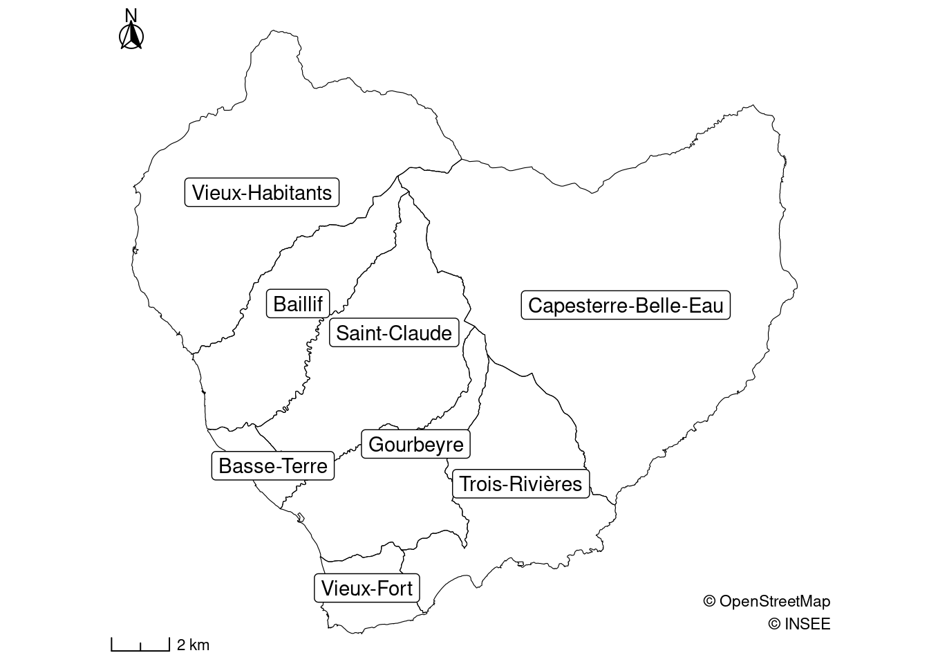
ggsave("data/map_premiere_carte.png", plot=map, width = 200, height = 200, units = "mm", dpi = "retina")Quelques statistiques descriptives avec GGPLOT2
Population communale
# Calculer la population pour chaque commune (somme de la population des IRIS)
pop_commune <- irisDfPop %>%
  group_by(LIBCOM) %>%
  summarise(P17_POP = sum(P17_POP))

# pop_commune
# Initialiser un graphique
c1 <- ggplot()+
geom_col(data = pop_commune, aes(x=LIBCOM,y=P17_POP))
# c1
# Ajouter un theme GGPLOT2, un titre, un sous-titre ...
c1 <- ggplot()+
geom_col(data = pop_commune, aes(x=LIBCOM,y=P17_POP))+
labs(title="Population communale (2017)", subtitle = "Huit communes, parmi les onze communes de la communauté d'agglomération",
caption = 'Données \u00a9 INSEE',x='Communes', y="Population")+
theme_bw()
# c1
# Modifier l'orientation du texte sur l'axe des abscisse
c1 <- ggplot()+
geom_col(data = pop_commune, aes(x=LIBCOM,y=P17_POP))+
labs(title="Population communale (2017)", subtitle = "Huit communes, parmi les onze communes de la communauté d'agglomération",
caption = 'Données \u00a9 INSEE',x='', y="Population")+
theme_bw() +
theme(axis.text.x = element_text(angle = 45, hjust=1))
# c1
# Modifier la couleur des barres
c1 <- ggplot()+
geom_col(data = pop_commune, aes(x=LIBCOM,y=P17_POP), fill="#e8833a", col="black")+
labs(title="Population communale (2017)", subtitle = "Huit communes, parmi les onze communes de la communauté d'agglomération",
caption = 'Données \u00a9 INSEE',x='', y="Population")+
theme_bw() +
theme(axis.text.x = element_text(angle = 45, hjust=1))
c1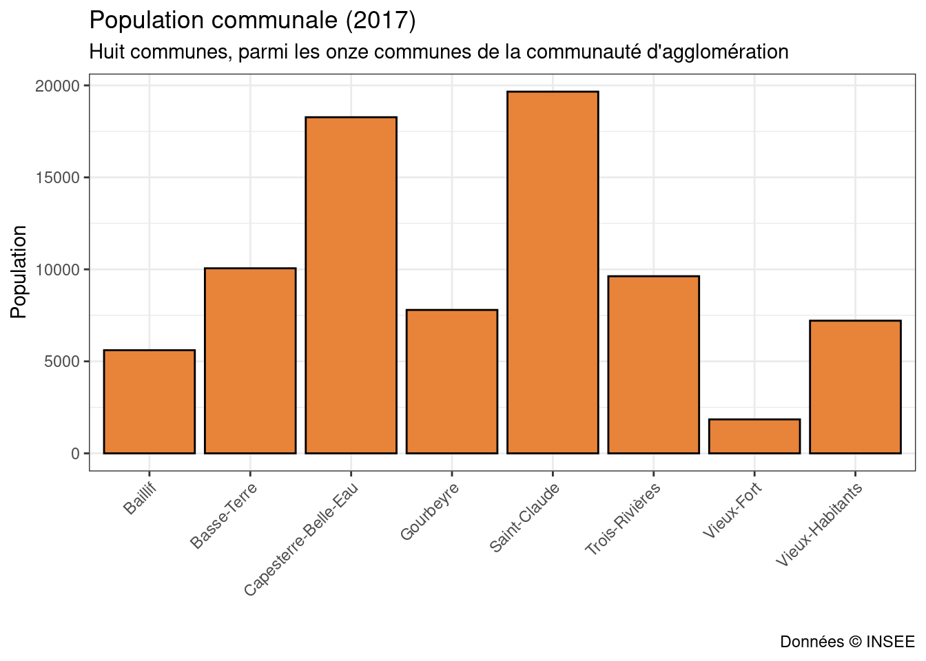
ggsave("data/population_communale_2017.png", plot=c1, width = 200, height = 200, units = "mm", dpi = "retina")# Jointure attributaire (carte population par commune)
communes_centroid <- communes %>%
merge(pop_commune, by.x="NOM", by.y="LIBCOM") %>%
st_centroid()
map <- ggplot() +
geom_sf(data = communes, col='black',fill='white')+
geom_sf_label(data = communes, aes(label = NOM))+
geom_sf(data = communes_centroid, aes(size=P17_POP), fill='#e8833a')+
annotation_scale(style='ticks',width_hint=0.1)+
annotation_north_arrow(style = north_arrow_fancy_orienteering,
height = unit(.75,"cm"),
width = unit(.75,"cm"),
location = "tl", which_north = "true")+
annotate('text', x = Inf, y = -Inf, label = '\u00a9 OpenStreetMap\n\u00a9 INSEE',
hjust = 1, vjust = -1, color = 'black', size = 3) +
theme_void()+
theme(legend.position = "right")
map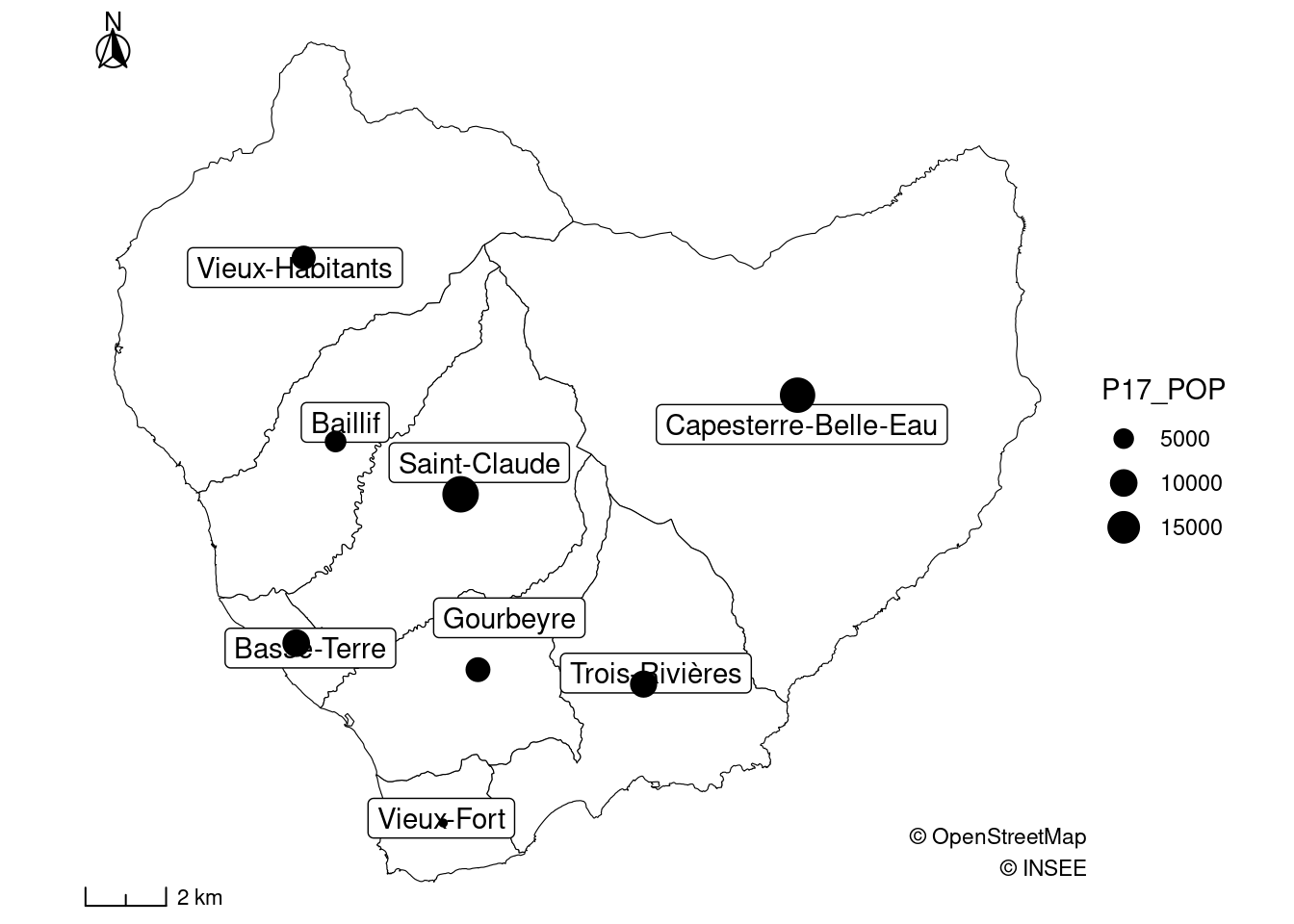
ggsave("carte_population.png", plot=map, width = 200, height = 200, units = "mm", dpi = "retina")df <- data.frame(ANNEE=c("1961","1967","1974","1982","1990","1999","2006","2011","2016","2019"),POP=c(13978,15690,15457,13656,14003,12410,12834,11730,10226,9861))
c1 <- ggplot()+
geom_line(data = df, aes(x=ANNEE,y=POP),col="#e8833a", group=1)+
geom_point(data = df, aes(x=ANNEE,y=POP),fill="#e8833a", col="black")+
ylim(0, 17000)+
labs(title="Evolution temporelle (1961-2019)", subtitle = "Population de la commune de Basse-Terre",
caption = 'Données \u00a9 INSEE',x='', y="Population")+
theme_bw() +
theme(axis.text.x = element_text(angle = 45, hjust=1))
c1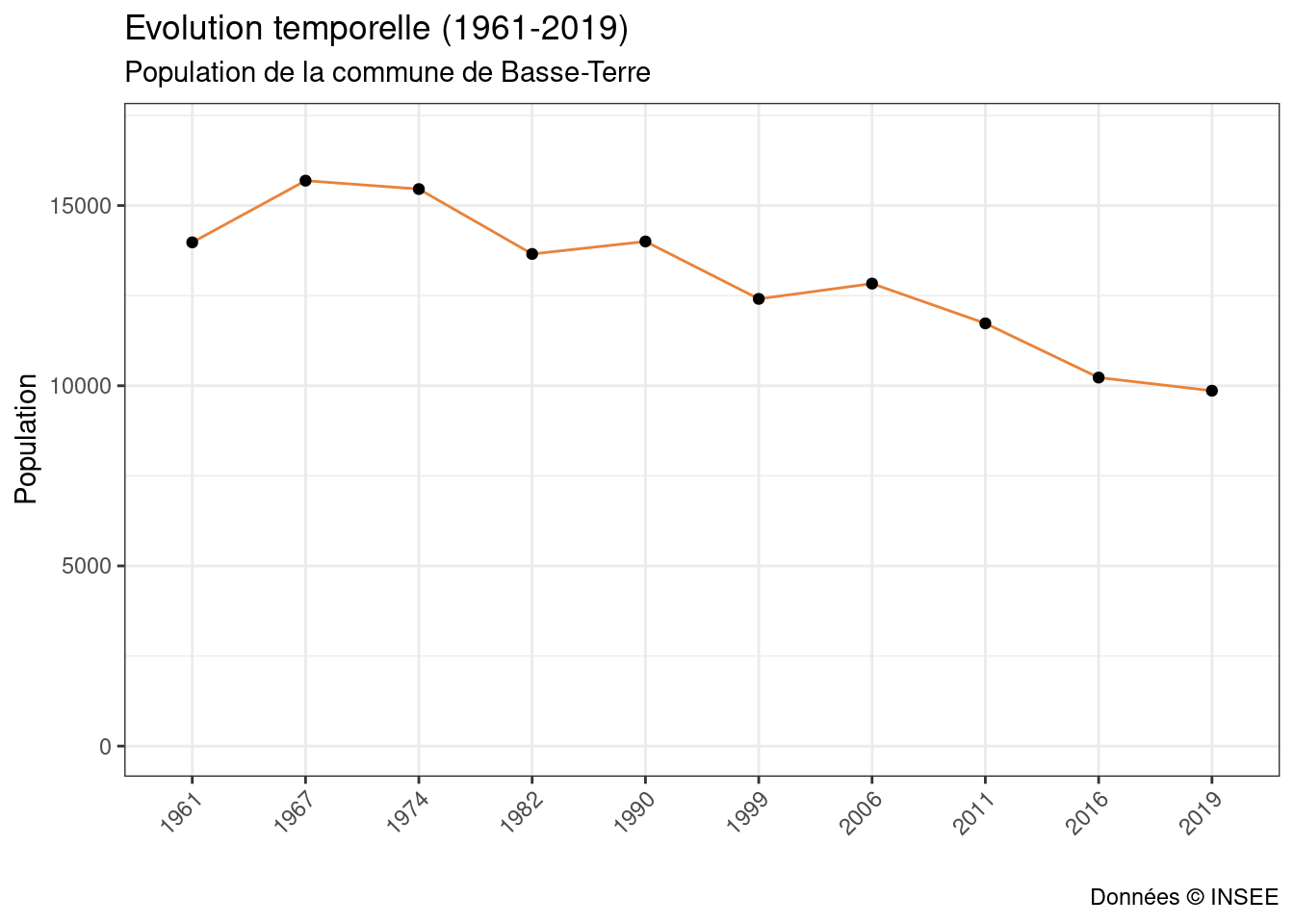
Mode de transport pour se rendre au travail
# Moyen de transport pour se rendre au travail
transport_commune <- irisDfAct %>%
  select("LIBCOM","C17_ACTOCC15P_PAS", "C17_ACTOCC15P_MAR", "C17_ACTOCC15P_VELO", "C17_ACTOCC15P_2ROUESMOT", "C17_ACTOCC15P_VOIT", "C17_ACTOCC15P_TCOM") %>%
  group_by(LIBCOM) %>%
  summarize(C17_ACTOCC15P_PAS = sum(C17_ACTOCC15P_PAS),
            C17_ACTOCC15P_MAR = sum(C17_ACTOCC15P_MAR),
            C17_ACTOCC15P_VELO = sum(C17_ACTOCC15P_VELO),
            C17_ACTOCC15P_2ROUESMOT = sum(C17_ACTOCC15P_2ROUESMOT),
            C17_ACTOCC15P_VOIT = sum(C17_ACTOCC15P_VOIT),
            C17_ACTOCC15P_TCOM = sum(C17_ACTOCC15P_TCOM))

colnames(transport_commune) <- c("LIBCOM","SANS_TRANSPORT", "PIETON","VELO","MOTO","VOITURE","TRANSPORT_COMMUN")

transport_Basse_Terre <- transport_commune %>%
  filter(LIBCOM=="Basse-Terre") %>%
  gather(., MODE, FREQ, -LIBCOM)

c1 <- ggplot()+
  geom_col(data = transport_Basse_Terre, aes(x=MODE,y=FREQ, fill=MODE), col="black")+
  labs(title="Mode de transport (Basse-Terre, 2017)", subtitle = "Nombre d'actifs occupés de 15 ans ou plus pour se rendre au travail",
       caption = 'Données \u00a9 INSEE',x='', y="Nombre d'individus")+
  theme_bw() +
  theme(axis.text.x =element_blank())
c1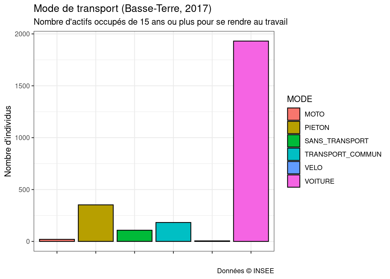
ggsave("transport_Basse_Terre_2017.png", plot=c1, width = 200, height = 200, units = "mm", dpi = "retina")transport_commune_by_commune <- transport_commune %>%
gather(., MODE, FREQ, -LIBCOM) %>%
mutate(LIBCOM=as.factor(LIBCOM))
c1 <- ggplot()+
geom_col(data = transport_commune_by_commune, aes(x=LIBCOM,y=FREQ, fill=MODE), col="black", position = "dodge")+
labs(title="Mode de transport (par commune en 2017)", subtitle = "Nombre d'actifs occupés de 15 ans ou plus pour se rendre au travail",
caption = 'Données \u00a9 INSEE',x='', y="Nombre d'individus")+
theme_bw() +
theme(axis.text.x = element_text(angle = 45, hjust=1))
c1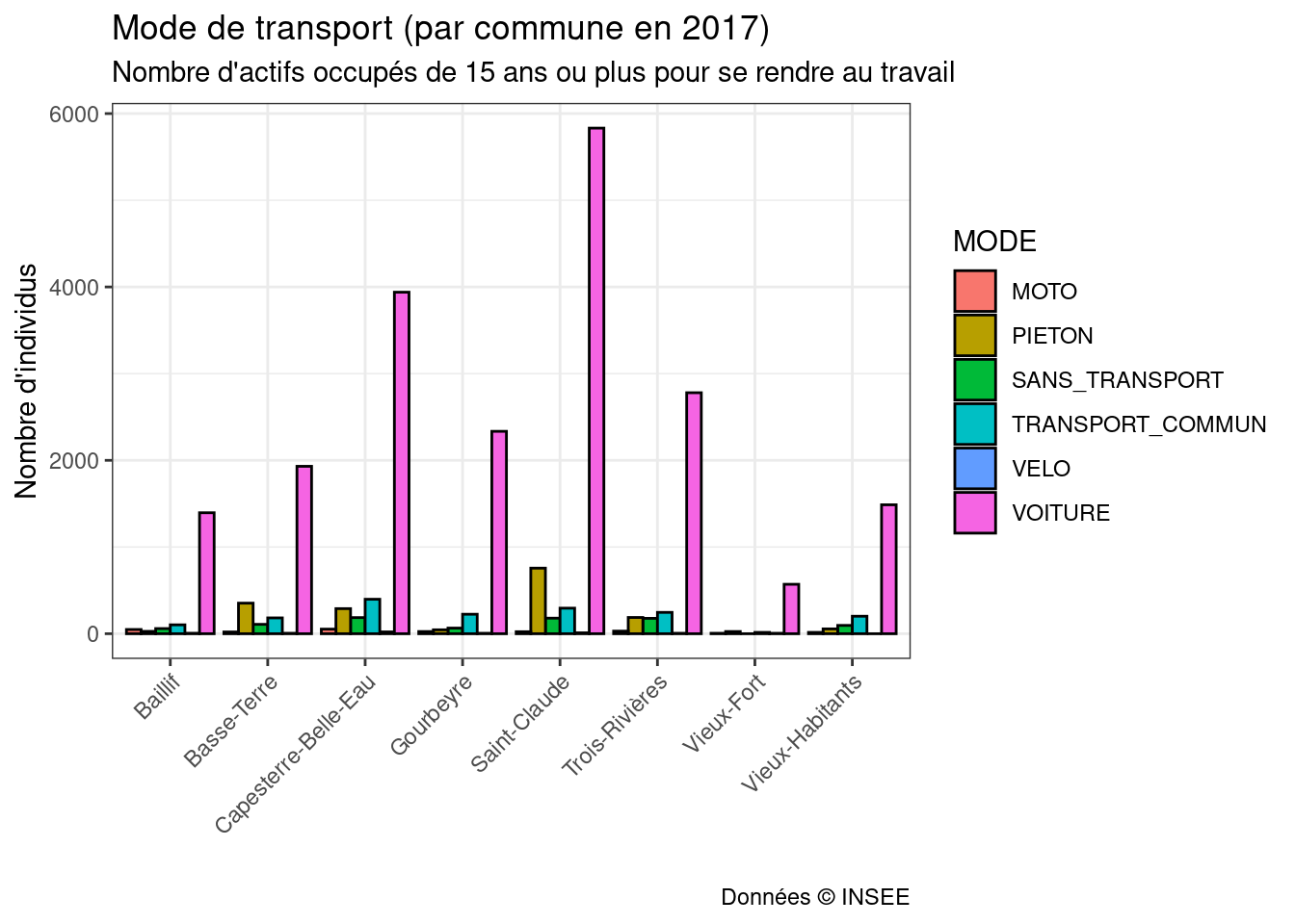
c1 <- ggplot()+
  geom_col(data = transport_commune_by_commune, aes(x=MODE,y=FREQ, fill=MODE), col="black", position = "dodge")+
  labs(title="Mode de transport (2017)", subtitle = "Nombre d'actifs occupés de 15 ans ou plus pour se rendre au travail",
       caption = 'Données \u00a9 INSEE',x='', y="Nombre d'individus")+
  facet_wrap(~LIBCOM)+
  theme_bw() +
  theme(axis.text.x = element_text(angle = 45, hjust=1))
c1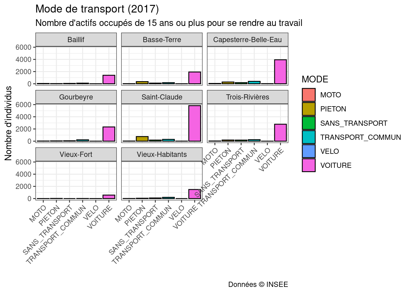
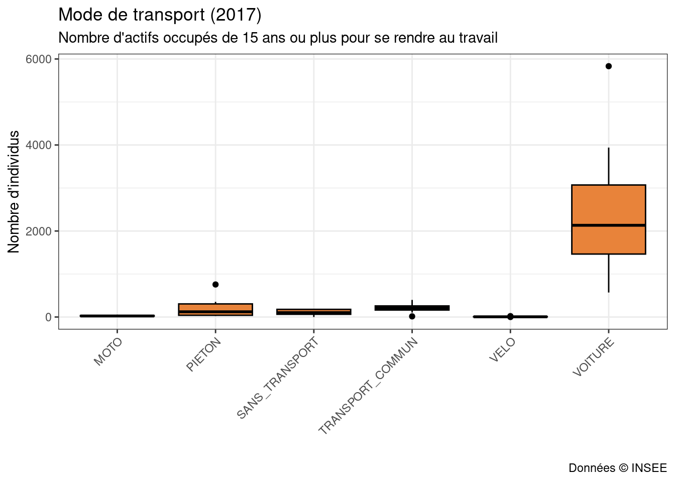
c1 <- ggplot()+
  geom_boxplot(data = transport_commune_by_commune, aes(x=MODE,y=FREQ), fill="#e8833a", col="black")+
  labs(title="Mode de transport (2017)", subtitle = "Nombre d'actifs occupés de 15 ans ou plus pour se rendre au travail",
       caption = 'Données \u00a9 INSEE',x='', y="Nombre d'individus")+
  theme_bw() +
  theme(axis.text.x = element_text(angle = 45, hjust=1))
c1